Introduction

Time complexity describes how the number of operations performed by an algorithm changes as the input size increases. Different algorithms can require different amounts of work for the same input. An algorithm may work efficiently for a small input but require significantly more operations as the input becomes larger.
Time complexity provides a way to describe this growth without depending on the exact execution time of a particular computer. Instead, it focuses on how the algorithm's work grows relative to the input size.
Some commonly used time complexities are O(1), O(log n), O(√n), O(n), O(n log n), O(n²), O(2ⁿ), and O(n!).
Understanding these growth rates helps developers analyze algorithms and choose approaches that can handle larger inputs efficiently.

Table of Contents

---

Constant Time Complexity - O(1)

Constant time complexity means that an algorithm performs approximately the same amount of work regardless of how large the input becomes.
The algorithm may receive 10 elements, 1,000 elements, or 1,000,000 elements, but the number of operations required for the particular task remains approximately constant.

Example:

numbers = [10, 20, 30, 40, 50]
first = numbers[0]
print(first)

The program directly accesses the first element using its index. It does not need to examine the remaining elements.
Whether the list contains 5 elements or 5 million elements, accessing an element by its index takes approximately the same amount of work.
Therefore, the time complexity is O(1). The amount of work remains approximately constant as the input size increases.

Example 2:

result = a + b
print(result)

The addition is a fixed operation for the purpose of basic algorithm analysis, so its time complexity is O(1).

Common examples:

• Accessing an element by index
• Assigning a value to a variable
• Performing a simple arithmetic operation
• Checking a single condition
• Accessing a value directly from a suitable hash-based structure

Constant time is generally considered highly scalable because increasing the input size does not cause the number of operations to grow with the input.

Logarithmic Time Complexity- O(log n)

Logarithmic time complexity occurs when an algorithm repeatedly reduces the amount of data that still needs to be processed.
A common example is binary search. Instead of checking every element, binary search examines the middle element and eliminates approximately half of the remaining search space after each comparison.
For binary search to work correctly, the data must be arranged in a suitable sorted order.

Example:

while left <= right:
    mid = (left + right) // 2
    if numbers[mid] == target:
        return mid
    elif numbers[mid] < target:
        left = mid + 1
    else:
        right = mid - 1

Suppose the search space contains 16 elements. The algorithm can reduce the search space approximately as follows:

16 to 8 to 4 to 2 to 1

Each step removes approximately half of the remaining elements. This means the algorithm does not need to inspect all 16 elements individually.
For a much larger input, the number of steps still increases slowly. For example, repeatedly dividing 1,024 elements by two takes only about 10 divisions to reach one element.
Therefore, binary search has a time complexity of O(log n).

Common examples:

• Binary search
• Searching in balanced search trees
• Algorithms that repeatedly divide a problem into smaller parts

Logarithmic algorithms are useful when dealing with large inputs because the amount of additional work grows slowly compared with the input size.

Square Root Time Complexity - O(√n)

Square root time complexity occurs when the number of operations grows approximately in proportion to the square root of the input size. It grows more slowly than linear time because √n is much smaller than n for large values of n.

Example:

i = 1
while i * i <= n:
    print(i)
    i += 1

The loop continues while i² is less than or equal to n.
For example, if n is 100, the loop runs while i is from 1 through 10 because:

10² = 100

Therefore, the number of iterations is approximately √n, giving the algorithm a time complexity of O(√n).
This type of complexity can appear in algorithms involving factors, divisors, and mathematical searches.
Although O(√n) is less common in basic algorithm examples than O(1), O(log n), O(n), and O(n²), it is useful to recognize when analyzing mathematical algorithms.

Linear Time Complexity - O(n)

Linear time complexity means that the amount of work grows proportionally with the input size.
If an algorithm processes every element of a collection once, the number of operations generally increases as the number of elements increases.

Example:

for number in numbers:
    print(number)

If the collection contains n elements, the loop executes approximately n times. If the input contains 10 elements, the loop processes approximately 10 elements. If the input contains 1,000 elements, it processes approximately 1,000 elements. Therefore, the time complexity is O(n).
If the input size doubles, the amount of work generally doubles as well.

Linear search is another common example.

for number in numbers:
    if number == target:
        return True
return False

The algorithm may need to inspect every element before finding the target or determining that the target is not present. Therefore, its worst-case time complexity is O(n).

Common examples:

• Traversing a list
• Linear search
• Counting elements
• Finding a maximum or minimum by checking every element
• Processing every item in a collection once

Linearithmic Time Complexity - O(n log n)

Linearithmic time complexity combines linear and logarithmic growth. It commonly appears in algorithms that divide a problem into smaller parts and then process all or most of the elements across multiple levels.
A common example is Merge Sort.
Merge Sort repeatedly divides a collection into smaller parts until the individual parts contain one element. It then combines those parts while maintaining sorted order.

Conceptually:

1.Divide the input 
2.Process the parts
3.Combine the results

The division creates approximately log n levels. At each level, approximately n elements are processed while the smaller parts are combined.

This gives:

n × log n = O(n log n)

Example:

def merge_sort(numbers):
    if len(numbers) <= 1:
        return numbers
    mid = len(numbers) // 2
    left = merge_sort(numbers[:mid])
    right = merge_sort(numbers[mid:])
    return merge(left, right)

The complete implementation of Merge Sort also requires a merge operation, but the important idea for complexity analysis is that the input is repeatedly divided while the elements are processed across the resulting levels.
Therefore, Merge Sort has a time complexity of O(n log n) in its standard analysis.

Common examples:

• Merge Sort
• Heap Sort
• Many efficient comparison-based sorting algorithms

O(n log n) grows faster than O(n), but much more slowly than O(n²) for large inputs.

Quadratic Time Complexity - O(n²)

Quadratic time complexity occurs when the amount of work grows approximately with the square of the input size.
A common way for an algorithm to have quadratic complexity is through two nested loops where each loop performs approximately n iterations.

Example:

for i in range(n):
    for j in range(n):
        print(i, j)

The outer loop executes n times. For every iteration of the outer loop, the inner loop also executes n times.

n × n = n²

Therefore, the total number of iterations is approximately n^2, and the time complexity is O(n²).
For example, if n is 100, the nested loops perform approximately 10,000 iterations. If n increases to 1,000, they perform approximately 1,000,000 iterations.

Example 2:

for i in range(n):
    for j in range(i + 1, n):
        print(i, j)

Although the exact number of iterations is less than n², it still grows proportionally to n². Therefore, its time complexity is O(n²).

Common examples:

• Comparing every pair of elements
• Two dependent nested loops
• Some simple sorting algorithms such as Bubble Sort and Selection Sort

Quadratic algorithms can become significantly slower as the input grows because the number of operations increases much faster than the input size.

Exponential Time Complexity - O(2ⁿ)

Exponential time complexity occurs when the amount of work grows exponentially with the input size.
In an O(2ⁿ) algorithm, increasing the input size by one can approximately double the amount of work.
A simple recursive structure can demonstrate this behavior.

Example:

def count(n):
    if n == 0:
        return
    count(n - 1)
    count(n - 1)

For each value of n greater than zero, the function makes two recursive calls. Each of those calls can make two more calls.
This creates a rapidly expanding recursion tree.
For example, the number of calls can grow approximately as:

1 to 2 to 4 to 8 to 16 ...

This growth pattern is exponential, so the time complexity of this recursive structure is O(2ⁿ).
Exponential algorithms can become impractical even for relatively moderate input sizes.

Common situations where exponential complexity can occur:

• Some recursive algorithms
• Generating all possible subsets
• Some brute-force solutions to combinatorial problems
• Recursive solutions that branch into multiple subproblems

Efficient algorithms often try to avoid unnecessary repeated work in exponential solutions by using techniques such as dynamic programming, memoization, or other problem-specific optimizations.

Factorial Time Complexity - O(n!)

Factorial time complexity occurs when the amount of work grows according to the factorial of the input size.
The factorial of n is calculated as:

n! = n × (n − 1) × (n − 2) × ... × 1

Factorial growth is extremely rapid. It increases even faster than exponential growth such as O(2ⁿ).
A common example is generating every possible permutation of n distinct elements.

Example:

from itertools import permutations
result = list(permutations(numbers))

If there are n distinct elements, there are exactly n! possible permutations. Therefore, the number of permutations grows as O(n!).

For example:

3! = 6
5! = 120
10! = 3,628,800

This shows how quickly the number of possibilities increases as n grows.
Factorial complexity commonly appears in brute-force problems where an algorithm needs to consider every possible ordering or arrangement.

Comparison of Common Time Complexities

The following table provides a quick comparison of the commonly encountered time complexities.

Complexity	Name	Typical Example
O(1)	Constant	Array index access
O(log n)	Logarithmic	Binary search
O(√n)	Square Root	Some divisor-search algorithms
O(n)	Linear	List traversal
O(n log n)	Linearithmic	Merge Sort
O(n2)	Quadratic	Nested loops
O(2n)	Exponential	Some recursive algorithms
O(n!)	Factorial	Generating permutations

The graph below shows how the different time complexities grow as the input size increases.

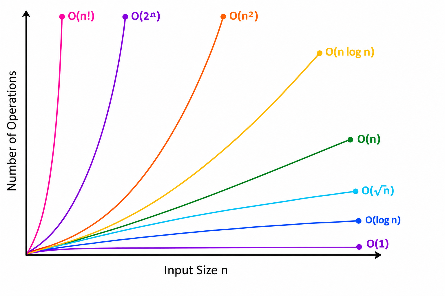
Figure: Comparison of common time complexity growth rates as the input size increases

How Growth Rates Compare

As the input size becomes larger, the difference between these complexities becomes increasingly significant.
In general, the growth rates can be ordered from slower to faster as:

O(1) < O(log n) < O(√n) < O(n) < O(n log n) < O(n²) < O(2ⁿ) < O(n!)

This ordering represents the general growth rate of these functions as n becomes large.

For example, O(n) grows more slowly than O(n²), while O(n²) grows more slowly than O(2ⁿ). This does not mean that an O(n) implementation will always run faster for every possible input. Actual performance can also depend on constant factors, implementation details, hardware, and the size of the input.
The important idea is that algorithms with faster-growing complexity require increasingly more work as the input becomes large.

Important Points to Remember

• O(1) remains approximately constant as n increases.
• O(log n) grows slowly because the problem size is repeatedly reduced.
• O(√n) grows slower than linear time.
• O(n) grows proportionally with the input size.
• O(n log n) commonly appears in efficient sorting algorithms.
• O(n²) commonly appears with two nested loops.
• O(2ⁿ) grows exponentially and can become expensive quickly.
• O(n!) grows extremely rapidly and commonly occurs when considering all permutations.
• Time complexity describes growth, not the exact number of seconds an algorithm takes.

Conclusion

Time complexity provides a way to understand how an algorithm's running time changes as the input size increases
.O(1) represents constant growth, while O(log n) grows slowly as the input increases. O(n) grows proportionally with the input, while O(n log n) is commonly found in efficient sorting algorithms. Polynomial complexities such as O(n²) and O(n³) can become expensive as the input grows. Exponential and factorial complexities such as O(2ⁿ) and O(n!) grow much more rapidly and can become impractical for larger inputs.
Understanding these common growth rates provides a foundation for analyzing algorithms, comparing solutions, and identifying approaches that can scale effectively with larger inputs.

Frequently Asked Questions (FAQs)

1. What is time complexity?

Time complexity describes how the amount of work performed by an algorithm changes as the input size increases.

2. What is O(1) time complexity?

O(1), or constant time, means that the amount of work remains approximately the same regardless of the input size.

3. What is O(log n) time complexity?

O(log n), or logarithmic time, occurs when an algorithm repeatedly reduces the amount of data that needs to be processed, such as in binary search.

4. What is O(n) time complexity?

O(n), or linear time, means that the amount of work grows approximately in proportion to the input size. Traversing every element of a list is a common example.

5. What is O(n log n) time complexity?

O(n log n), or linearithmic time, commonly occurs in efficient sorting algorithms such as Merge Sort.